Cleaning Data with stringr

Introduction

Occassionally, when we are using a set of data, there may be mistakes. Before we can really make any decisions or visualizations using that data, we must ensure it is as accurate as possible. In this post, we will look at using the R library stringr to filter out unwanted data.

Basic Example

For this example, we will be using a data set from (Kaggle.com)[https://www.kaggle.com/orangutan/exploratory-analysis-of-the-korean-war] that contains all the US deaths from the Korean War. First, we import our libraries and look at the first few rows of data.

library(dplyr)
library(stringr)

#read in the data
deaths<-read.csv("KoreanConflict.csv", header=TRUE, stringsAsFactors=FALSE)

head(deaths)

##   SERVICE_TYPE SERVICE_CODE             ENROLLMENT    BRANCH RANK
## 1            V            L ACTIVE - GUARD/RESERVE AIR FORCE CAPT
## 2            R            K       ACTIVE - REGULAR      ARMY  PVT
## 3            R            K       ACTIVE - REGULAR      ARMY  PFC
## 4            V            L ACTIVE - GUARD/RESERVE      ARMY  2LT
## 5            R            K       ACTIVE - REGULAR      ARMY  CPL
## 6            R            K       ACTIVE - REGULAR      ARMY  PFC
##   PAY_GRADE                      POSITION BIRTH_YEAR SEX HOME_CITY
## 1       O03                                     1917   M  NEW YORK
## 2       E02       FOOD SERVICE APPRENTICE       1927   M   UNKNOWN
## 3       E03     HEAVY WEAPONS INFANTRYMAN       1932   M   UNKNOWN
## 4       O01       INFANTRY UNIT COMMANDER       1929   M   UNKNOWN
## 5       E04 LIGHT WEAPONS INFANTRY LEADER       1932   M   UNKNOWN
## 6       E03     LIGHT WEAPONS INFANTRYMAN       1929   M   UNKNOWN
##   HOME_COUNTY NATIONALITY STATE_CODE   HOME_STATE MARITAL_STATUS ETHNICITY
## 1    NEW YORK          US         NY     NEW YORK        MARRIED     WHITE
## 2      OCONEE          US         GA      GEORGIA        UNKNOWN     WHITE
## 3        BIBB          US         GA      GEORGIA        UNKNOWN     WHITE
## 4     COAHOMA          US         MS  MISSISSIPPI        UNKNOWN     WHITE
## 5      DICKEY          US         ND NORTH DAKOTA        UNKNOWN     WHITE
## 6      NELSON          US         ND NORTH DAKOTA        UNKNOWN     WHITE
##     ETHNICITY_1 ETHNICITY_2              DIVISION INCIDENT_DATE
## 1 NOT SPECIFIED       WHITE 93 BOMB SQ 19 BOMB GP      19510412
## 2 NOT SPECIFIED       WHITE      29 RGT CMBT TEAM      19500727
## 3 NOT SPECIFIED       WHITE       5 RGT 1 CAV DIV      19510316
## 4 NOT SPECIFIED       WHITE          32 INF 7 DIV      19530122
## 5 NOT SPECIFIED       WHITE         14 INF 25 DIV      19530529
## 6 NOT SPECIFIED       WHITE       5 RGT 1 CAV DIV      19510606
##   FATALITY_YEAR FATALITY_DATE HOSTILITY_CONDITIONS         FATALITY
## 1          1951      20010402                    H    DECLARED DEAD
## 2          1950      19500727                    H KILLED IN ACTION
## 3          1951      19510316                    H KILLED IN ACTION
## 4          1953      19530122                    H KILLED IN ACTION
## 5          1953      19530529                    H KILLED IN ACTION
## 6          1951      19510606                    H KILLED IN ACTION
##   BURIAL_STATUS
## 1             Y
## 2             Y
## 3             Y
## 4             Y
## 5             Y
## 6             Y

It appears that the INCIDENT_DATE field is formatted like so: YYYYMMDD. To check this, let’s compare the total number of rows in the database with how many rows fit that format. To keep things simple, we will use a regular expression to check that the data contains only 8 numbers.

#Get the total number of records int the data
count(deaths) #36,574

## # A tibble: 1 x 1
##       n
##   <int>
## 1 36574

#compare INCIDENT_DATE against the regular expression and get the count of records
fullDateRegEx = "^\\d{8}$"

df<-deaths%>%
  filter(str_detect(deaths$INCIDENT_DATE, fullDateRegEx)==TRUE)
count(df) #33,370

## # A tibble: 1 x 1
##       n
##   <int>
## 1 33370

Looking further into the data, we can see that the FATALITY column also appears to hold a date in the format we want, and only shows that when INCIDENT_DATE is invalid. Using a simple for loop, we can check to see if FATALITY is valid when INCIDENT_DATE is not, and store the date in INCIDENT_DATE

for (i in 1:dim(deaths)) {
  #if INCIDENT_DATE is bad, but FATALITY is good, replace it
  if (!str_detect(deaths$INCIDENT_DATE[i], fullDateRegEx) & str_detect(deaths$FATALITY[i], fullDateRegEx)) {
    #print(paste(i, "There is a mistake here"))
    deaths$INCIDENT_DATE[i]<-deaths$FATALITY[i]
  }
}

## Warning in 1:dim(deaths): numerical expression has 2 elements: only the
## first used

#Check out counts again
df<-deaths%>%
  filter(str_detect(deaths$INCIDENT_DATE, fullDateRegEx)==TRUE)
count(df) #36,511

## # A tibble: 1 x 1
##       n
##   <int>
## 1 36511

This is an acceptable number of valid records (36,511 out of 36,574), so we can just filter out the remaining bad data and begin to use our data for visualizations and decision making.

deaths<-deaths%>%
  filter(str_detect(deaths$INCIDENT_DATE, fullDateRegEx)==TRUE)

Visualization

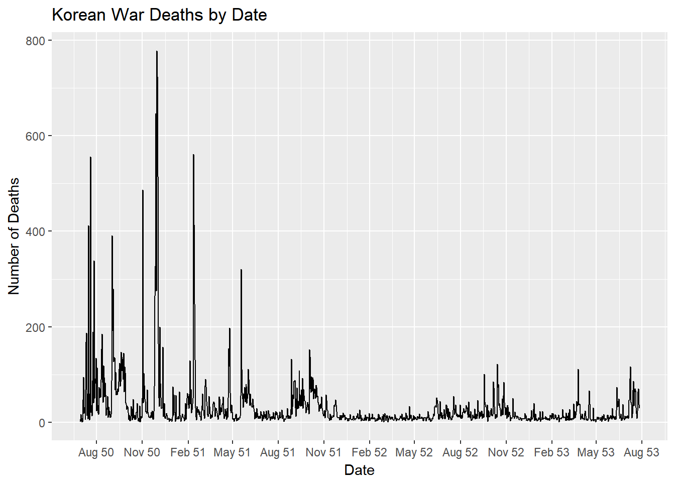
Now we can plot out a simple line chart of deaths by date using this newly cleaned data set.

library(ggplot2)
library(lubridate)  #for parsing and dealing with dates

deathsDf<-deaths%>%
  group_by(INCIDENT_DATE)%>%
  summarize(num_deaths=n())%>%
  mutate(date=ymd(INCIDENT_DATE))%>%
  filter(date<='1953-07-27')%>%
  select(INCIDENT_DATE, date, num_deaths)

#look at number of deaths by date
ggplot()+
  geom_line(data=deathsDf, aes(x=date,y=num_deaths))+
  ggtitle("Korean War Deaths by Date")+
  xlab("Date")+
  ylab("Number of Deaths")+
  scale_x_date(date_breaks="3 months", date_labels="%b %y")