Combining Multiple Wordclouds into one
Introduction
In the previous post titled “Simple Sentiment Analysis”, we plotted both positive and negative words onto one line chart. In “Using ggplot - Introduction to facet_wrap()”, we combined two different bar charts into one plot, but positive and negative words were separated. In this example, we will do something similar, but with wordclouds.
Getting Data to Analyze
We have previously built a wordcloud using Jane Austen’s novel “Sense & Sensibility”, but for this example, will continue using Bram Stoker’s “Dracula” to create a positive and negative wordcloud. For a more indepth explanation of how we get this data, please see the post “Simple Sentiment Analysis”.
library(gutenbergr)
library(tidytext)
library(dplyr)
library(wordcloud)

dracula<-gutenberg_download(345)
dracula$gutenberg_id<-NULL

dracula<-dracula%>%
  unnest_tokens(word, text)

bing<-get_sentiments('bing')
dracula<-inner_join(dracula, bing)
Organizing our Data
Now that we have a dataframe of all the words from “Dracula” joined with the words in the Bing lexicon, we need to count up the number of times each word occurs, but we need to keep the sentiment in tact for each word. A simple addition to the summarize() method in dplyr will add that to our grouping. The first() function will pick the first value of that column and use that for the column data.
words<-dracula%>%
  group_by(word)%>%
  summarize(count=n(), sentiment=first(sentiment))%>%
  arrange(count)

head(words)
## # A tibble: 6 x 3
## word count sentiment
## <chr> <int> <chr>
## 1 abnormal 1 negative
## 2 abyss 1 negative
## 3 accidental 1 negative
## 4 accursed 1 negative
## 5 aching 1 negative
## 6 acumen 1 positiveCreating the Wordcloud
Below, we create the wordcloud, but all the positive and negative words are combined together, which is not what we want. We want to be able to determine the sentiment easily when looking at the wordcloud.
wordcloud(words$word, words$count, max.words=150)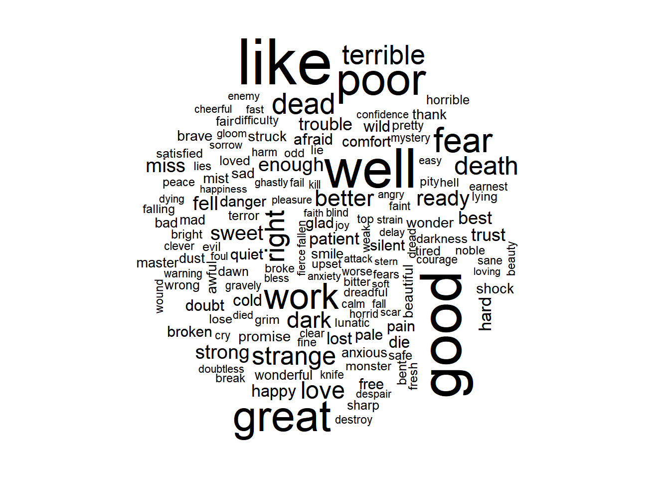
In order to do this comparison, we need a new library called reshape2. This library will allow us to turn our dataframe into a matrix, which is required to use wordcloud’s comparison cloud plot.
library(reshape2)
matrix<-acast(words, word~sentiment, value.var='count', fill=0)
Now that we have our matrix, creating the comparison cloud is just as easy as making a normal wordcloud.
comparison.cloud(matrix, colors=c('black', 'orange'))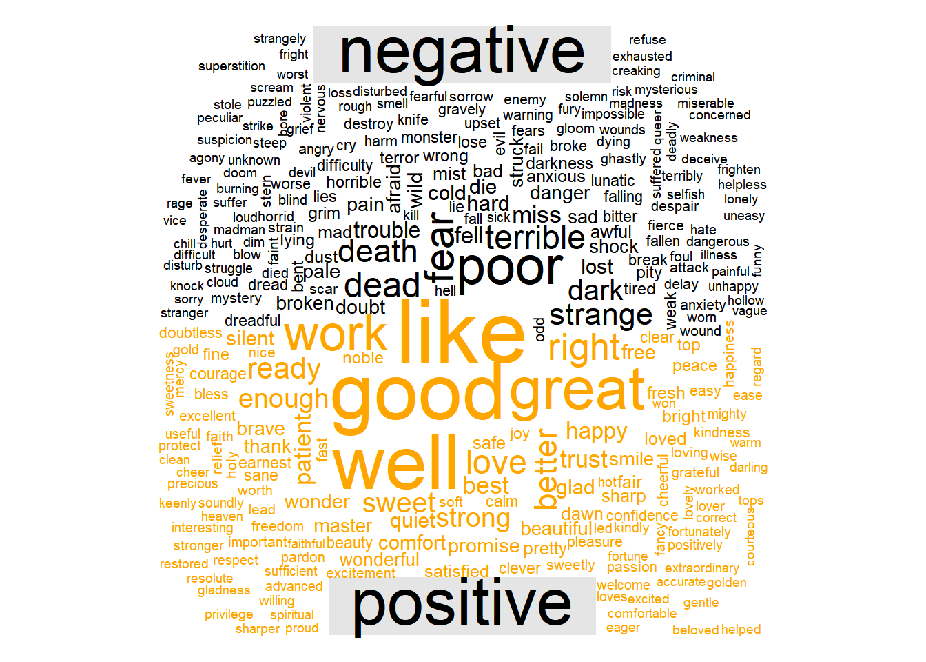
The Code
The code for this post can be found on my GitHub Gists page.