Simple Sentiment Analysis
Introduction
The tidytext package in R provides a few functions and dataframes for sentiment analysis. Sentiment analysis is a way to determine the “feeling” a word represents. For example, the word “abhor” gives a negative vibe to it, whereas “sunshine” gives a positive vibe. Additionally, the word “agonize” is more negative than “afflicted”.
Getting Data to Analyze
We will be using the gutenbergr package in R to get the text from the novel Frankenstein. To prepare our data for sentiment analysis we will split the lines of data into words. Finally, we will group the words into chunks of 80 lines, so as to analyze the sentiments in larger chunks.
library(dplyr)
library(tidytext)
library(gutenbergr)

dracula<-gutenberg_download(345)

# Remove unnecessary columns and give each row a line number
# Then split into words
dracula$gutenberg_id<-NULL
dracula$line<-1:15568
words<-dracula%>%
  unnest_tokens(word, text)
words$grouping<-words$line %/% 80
Bing Lexicon
The first lexicon we will look at is bing. This lexicon provides a list of words and rates it as either positive or negative. It is a simple way of determining the overall feeling of the next. Once we have the lexicon, we will it with our dataframe of words. This will create one dataframe with just the words from Dracula that are in the Bing lexicon.
bing<-get_sentiments('bing')
words_bing<-inner_join(words, bing)
Since there is no numerical score given for each word, we can assign +1 for positive and -1 for negative. This will help us later when we are trying to plot the overall value of each group of lines.
words_bing$score<-1
negrows<-which(words_bing$sentiment=='negative')
words_bing$score[negrows]<--1
Afinn Lexicon
Another lexicon we will look at is called afinn. This lexicon expands on bing a bit by assigning a numerical score to each word. Negative numbers are negative in sentiment, while positive numbers are positive. The larger the deviation from zero, the more severe the negativity or positivity. Since we already have a score for each word, we only need to join our words to the afinn lexicon.
afinn<-get_sentiments('afinn')
words_afinn<-inner_join(words, afinn)
Plotting the Data
Using ggplot2, we can plot a line chart of each lexicon to compare the scoring values for each group of 80 lines. First we must query our words to group each 80 lines, and sum up the total score.
sent_afinn<-words_afinn%>%
  group_by(grouping)%>%
  summarize(value=sum(score))

sent_bing<-words_bing%>%
  group_by(grouping)%>%
  summarize(value=sum(score))
Now, a simple line chart for both lexicon dataframes will compare the two values.
library(ggplot2)
ggplot()+
  geom_line(data=sent_afinn, aes(x=grouping,y=value), color='orange')+
  geom_line(data=sent_bing, aes(x=grouping,y=value), color='black')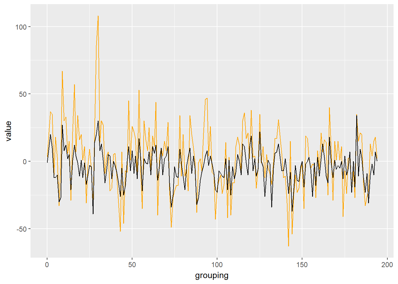
The Code
The code for this post can be found on my GitHub Gists page.